CDS-Bond Basis Replication: Project Tour

CDS-Bond Basis Replication: Project Tour#

This notebook is the high-level walkthrough of our CDS-bond basis replication workflow. It documents what we replicate, which data we use, the main pipeline steps, and the final outputs used in the report/site.

1. Replication Goal#

We focus on the CDS-bond basis component from Siriwardane, Sunderam, and Wallen’s Segmented Arbitrage:

Bond-level basis: cds_basis_spread = par_spread - z_spread
In basis points: cds_basis_spread_bps = cds_basis_spread * 10000

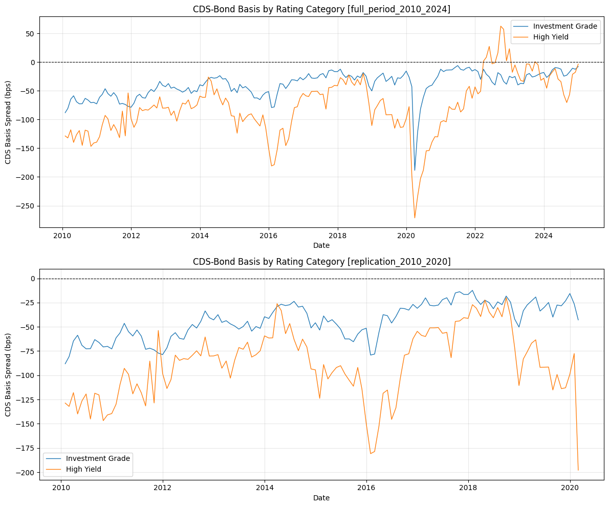
The objective is to produce clean bond-level and aggregated time series (Investment Grade vs High Yield), plus diagnostics and summary statistics.

2. Data Sources (Current Pipeline)#

WRDS Markit CDS (markit_cds.parquet)
- redcode, date, tenor, parspread
WRDS RED mapping (RED_and_ISIN_mapping.parquet)
- maps ISIN to RED entity code
WRDS bond returns (wrds_bondret_project.parquet)
- bond characteristics and pricing inputs
CRSP Treasury + Fed yield curve
- curve fitting for z-spread, with Fed fallback checks on problematic dates

Current final analysis files:

_data/cds_basis_processed.parquet
_data/cds_basis_aggregated.parquet
_data/cds_basis_non_aggregated.parquet
_data/cds_basis_summary_stats.csv

3. Pipeline Steps Implemented#

Pull and clean bond/CDS/mapping datasets.
Merge bonds to CDS entities via ISIN->REDCODE mapping.
Interpolate CDS par spreads at bond maturity horizon.
Estimate bond z-spreads from pricing equations.
Compute CDS-bond basis spread and aggregate by rating/date.
Export datasets, chart, and summary stats.

from pathlib import Path

import matplotlib.pyplot as plt
import pandas as pd
import seaborn as sns
import chartbook

BASE_DIR = chartbook.env.get_project_root()
DATA_DIR = BASE_DIR / "_data"

4. Load Final Processed Data#

agg_df = pd.read_parquet(DATA_DIR / "cds_basis_aggregated.parquet")
non_agg_df = pd.read_parquet(DATA_DIR / "cds_basis_non_aggregated.parquet")
stats_df = pd.read_csv(DATA_DIR / "cds_basis_summary_stats.csv")

print("=== Aggregated Dataset ===")
print(f"Shape: {agg_df.shape}")
print(f"Date range: {agg_df['date'].min()} to {agg_df['date'].max()}")
print(f"Rating buckets: {agg_df['c_rating'].unique().tolist()}")
if "analysis_period" in agg_df.columns:
    print(f"Analysis periods: {agg_df['analysis_period'].dropna().unique().tolist()}")

print("\n=== Non-Aggregated Dataset ===")
print(f"Shape: {non_agg_df.shape}")
print(f"Date range: {non_agg_df['date'].min()} to {non_agg_df['date'].max()}")
id_col = "isin" if "isin" in non_agg_df.columns else "cusip"
print(f"Unique IDs ({id_col}): {non_agg_df[id_col].nunique()}")

=== Aggregated Dataset ===
Shape: (604, 10)
Date range: 2010-01-31 00:00:00 to 2024-12-31 00:00:00
Rating buckets: ['High Yield', 'Investment Grade']
Analysis periods: ['replication_2010_2020', 'full_period_2010_2024']

=== Non-Aggregated Dataset ===
Shape: (204899, 10)
Date range: 2010-01-31 00:00:00 to 2024-12-31 00:00:00
Unique IDs (isin): 2243

5. Summary Statistics#

print("Project summary stats table:")
display(stats_df)

if "analysis_period" in agg_df.columns:
    for period in sorted(agg_df["analysis_period"].dropna().unique()):
        agg_wide = agg_df[agg_df["analysis_period"] == period].pivot(
            index="date", columns="c_rating", values="cds_basis_spread_bps"
        )
        print(f"\nAggregated CDS-bond basis spread (bps) by rating [{period}]:")
        display(agg_wide.describe().T)
else:
    agg_wide = agg_df.pivot(index="date", columns="c_rating", values="cds_basis_spread_bps")
    print("\nAggregated CDS-bond basis spread (bps) by rating:")
    display(agg_wide.describe().T)

print("\nBond-level CDS-bond basis spread stats (bps):")
display(non_agg_df["cds_basis_spread_bps"].describe())

Project summary stats table:

	group	n_obs	start_date	end_date	mean_bps	median_bps	std_bps	analysis_period	period_label	period_start	period_end
0	All bonds	122	2010-01-31	2020-02-29	-55.102355	-56.172446	21.139116	replication_2010_2020	Replication (2010-01-01 to 2020-02-29)	2010-01-01	2020-02-29
1	Investment Grade	122	2010-01-31	2020-02-29	-43.852373	-42.835425	18.198621	replication_2010_2020	Replication (2010-01-01 to 2020-02-29)	2010-01-01	2020-02-29
2	High Yield	122	2010-01-31	2020-02-29	-88.019349	-84.569900	35.462100	replication_2010_2020	Replication (2010-01-01 to 2020-02-29)	2010-01-01	2020-02-29
3	All bonds	180	2010-01-31	2024-12-31	-48.714874	-43.748939	28.092973	full_period_2010_2024	Full Period (2010-01-01 to 2024-12-31)	2010-01-01	2024-12-31
4	Investment Grade	180	2010-01-31	2024-12-31	-38.772864	-33.678487	23.191339	full_period_2010_2024	Full Period (2010-01-01 to 2024-12-31)	2010-01-01	2024-12-31
5	High Yield	180	2010-01-31	2024-12-31	-76.822096	-78.750047	50.625029	full_period_2010_2024	Full Period (2010-01-01 to 2024-12-31)	2010-01-01	2024-12-31

Aggregated CDS-bond basis spread (bps) by rating [full_period_2010_2024]:

	count	mean	std	min	25%	50%	75%	max
c_rating
High Yield	180.0	-76.822096	50.625029	-271.396379	-106.099087	-78.750047	-42.996925	62.555892
Investment Grade	180.0	-38.772864	23.191339	-188.552595	-51.731793	-33.678487	-22.808611	-6.104417

Aggregated CDS-bond basis spread (bps) by rating [replication_2010_2020]:

	count	mean	std	min	25%	50%	75%	max
c_rating
High Yield	122.0	-88.019349	35.462100	-197.885137	-113.457249	-84.569900	-61.745672	-19.913129
Investment Grade	122.0	-43.852373	18.198621	-88.114059	-56.272803	-42.835425	-27.605197	-12.370801

Bond-level CDS-bond basis spread stats (bps):

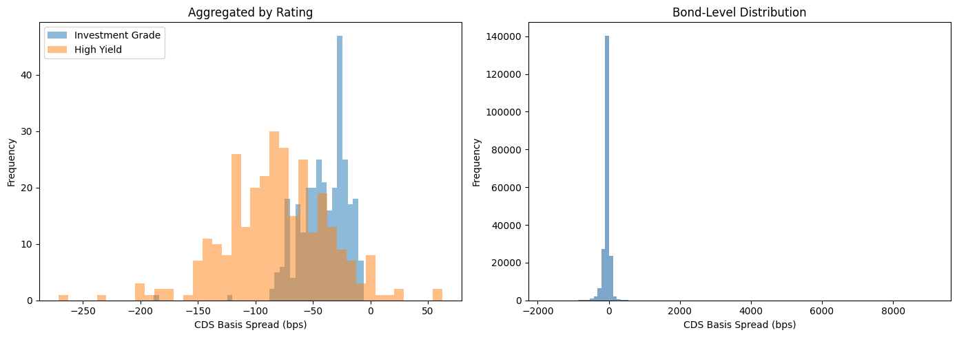
count    204899.000000
mean        -53.192067
std         107.441160
min       -1722.708802
25%         -81.288627
50%         -39.921375
75%         -11.960890
max        9084.999656
Name: cds_basis_spread_bps, dtype: float64

6. Time Series: Basis by Rating#

if "analysis_period" in agg_df.columns:
    periods = sorted(agg_df["analysis_period"].dropna().unique())
    fig, axes = plt.subplots(len(periods), 1, figsize=(12, 5 * len(periods)), sharex=False)
    if len(periods) == 1:
        axes = [axes]
    for ax, period in zip(axes, periods):
        g = agg_df[agg_df["analysis_period"] == period]
        for rating in ["Investment Grade", "High Yield"]:
            s = g[g["c_rating"] == rating].sort_values("date")
            ax.plot(s["date"], s["cds_basis_spread_bps"], label=rating, linewidth=1.0)
        ax.axhline(0, color="black", linewidth=0.8, linestyle="--")
        ax.set_xlabel("Date")
        ax.set_ylabel("CDS Basis Spread (bps)")
        ax.set_title(f"CDS-Bond Basis by Rating Category [{period}]")
        ax.legend(loc="best")
        ax.grid(True, alpha=0.3)
    plt.tight_layout()
    plt.show()
else:
    fig, ax = plt.subplots(figsize=(12, 6))
    for rating in ["Investment Grade", "High Yield"]:
        s = agg_df[agg_df["c_rating"] == rating].sort_values("date")
        ax.plot(s["date"], s["cds_basis_spread_bps"], label=rating, linewidth=1.0)

    ax.axhline(0, color="black", linewidth=0.8, linestyle="--")
    ax.set_xlabel("Date")
    ax.set_ylabel("CDS Basis Spread (bps)")
    ax.set_title("CDS-Bond Basis by Rating Category")
    ax.legend(loc="best")
    ax.grid(True, alpha=0.3)
    plt.tight_layout()
    plt.show()

../../_images/55dd85b95f2d92789ac0183023141821982b93b9e0663235c8fa9c128cfa7dd6.png

7. Distribution Checks#

fig, axes = plt.subplots(1, 2, figsize=(14, 5))
for rating in ["Investment Grade", "High Yield"]:
    subset = agg_df[agg_df["c_rating"] == rating]
    axes[0].hist(subset["cds_basis_spread_bps"], bins=40, alpha=0.5, label=rating)
axes[0].set_xlabel("CDS Basis Spread (bps)")
axes[0].set_ylabel("Frequency")
axes[0].set_title("Aggregated by Rating")
axes[0].legend()

axes[1].hist(non_agg_df["cds_basis_spread_bps"], bins=100, alpha=0.7, color="steelblue")
axes[1].set_xlabel("CDS Basis Spread (bps)")
axes[1].set_ylabel("Frequency")
axes[1].set_title("Bond-Level Distribution")

plt.tight_layout()
plt.show()

../../_images/e5c3a5a0ce13414f56a7c64d64cd33fd8eb7eb76cedee81ff11c348a4286d5da.png

8. Correlation Across Rating Buckets#

if "analysis_period" in agg_df.columns:
    for period in sorted(agg_df["analysis_period"].dropna().unique()):
        agg_wide = agg_df[agg_df["analysis_period"] == period].pivot(
            index="date", columns="c_rating", values="cds_basis_spread_bps"
        )
        if len(agg_wide.columns) > 1:
            corr_matrix = agg_wide.corr()
            print(f"Correlation matrix [{period}]:")
            display(corr_matrix)

            fig, ax = plt.subplots(figsize=(6, 5))
            sns.heatmap(corr_matrix, annot=True, cmap="coolwarm", center=0, ax=ax)
            ax.set_title(f"Correlation: CDS-Bond Basis Spread by Rating [{period}]")
            plt.tight_layout()
            plt.show()
else:
    if len(agg_wide.columns) > 1:
        corr_matrix = agg_wide.corr()
        print("Correlation matrix:")
        display(corr_matrix)

        fig, ax = plt.subplots(figsize=(6, 5))
        sns.heatmap(corr_matrix, annot=True, cmap="coolwarm", center=0, ax=ax)
        ax.set_title("Correlation: CDS-Bond Basis Spread by Rating")
        plt.tight_layout()
        plt.show()

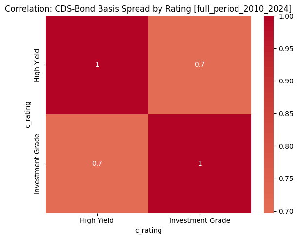
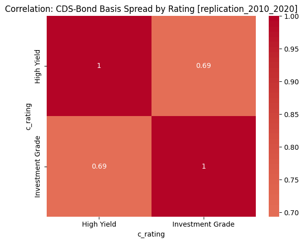
Correlation matrix [full_period_2010_2024]:

c_rating	High Yield	Investment Grade
c_rating
High Yield	1.00000	0.69696
Investment Grade	0.69696	1.00000

../../_images/ddfbba9772b5b4d9108dbaf8a3a3d4f1fee7e260414530b8002dcb080086daa5.png

Correlation matrix [replication_2010_2020]:

c_rating	High Yield	Investment Grade
c_rating
High Yield	1.000000	0.693878
Investment Grade	0.693878	1.000000

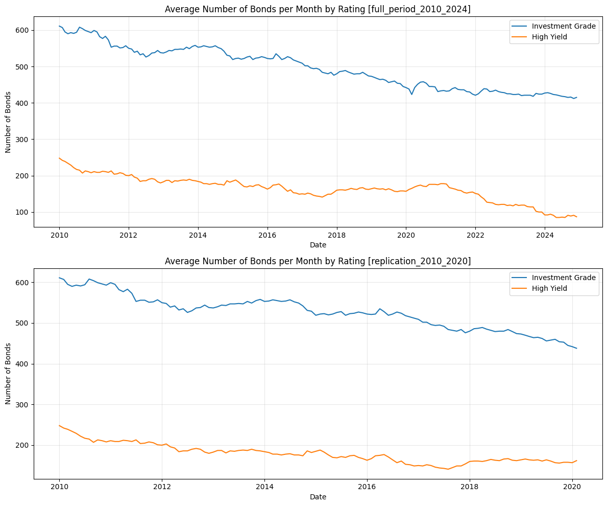
../../_images/3da7b16917bcf0b0927b0a2345b3f5ae2f3318d1d73729192512903de2edf26a.png

9. Monthly Counts and Data Quality#

agg_df["date"] = pd.to_datetime(agg_df["date"])
if "analysis_period" in agg_df.columns:
    periods = sorted(agg_df["analysis_period"].dropna().unique())
    fig, axes = plt.subplots(len(periods), 1, figsize=(12, 5 * len(periods)), sharex=False)
    if len(periods) == 1:
        axes = [axes]
    for ax, period in zip(axes, periods):
        g = agg_df[agg_df["analysis_period"] == period]
        monthly_counts = (
            g.groupby([g["date"].dt.to_period("M"), "c_rating"])["n_bonds"]
            .mean()
            .reset_index()
        )
        monthly_counts["date"] = monthly_counts["date"].dt.to_timestamp()
        for rating in ["Investment Grade", "High Yield"]:
            s = monthly_counts[monthly_counts["c_rating"] == rating]
            ax.plot(s["date"], s["n_bonds"], label=rating)
        ax.set_title(f"Average Number of Bonds per Month by Rating [{period}]")
        ax.set_xlabel("Date")
        ax.set_ylabel("Number of Bonds")
        ax.grid(alpha=0.3)
        ax.legend()
    plt.tight_layout()
    plt.show()
else:
    monthly_counts = (
        agg_df.groupby([agg_df["date"].dt.to_period("M"), "c_rating"])["n_bonds"]
        .mean()
        .reset_index()
    )
    monthly_counts["date"] = monthly_counts["date"].dt.to_timestamp()

    fig, ax = plt.subplots(figsize=(12, 5))
    for rating in ["Investment Grade", "High Yield"]:
        s = monthly_counts[monthly_counts["c_rating"] == rating]
        ax.plot(s["date"], s["n_bonds"], label=rating)
    ax.set_title("Average Number of Bonds per Month by Rating")
    ax.set_xlabel("Date")
    ax.set_ylabel("Number of Bonds")
    ax.grid(alpha=0.3)
    ax.legend()
    plt.tight_layout()
    plt.show()

print("Missing values (aggregated bps):", agg_df["cds_basis_spread_bps"].isna().sum())
print("Missing values (non-aggregated bps):", non_agg_df["cds_basis_spread_bps"].isna().sum())

../../_images/59ead5801e2630ad7dcc5b154c671315307ce4c60c756f06e5946c759f589b92.png

Missing values (aggregated bps): 0
Missing values (non-aggregated bps): 0

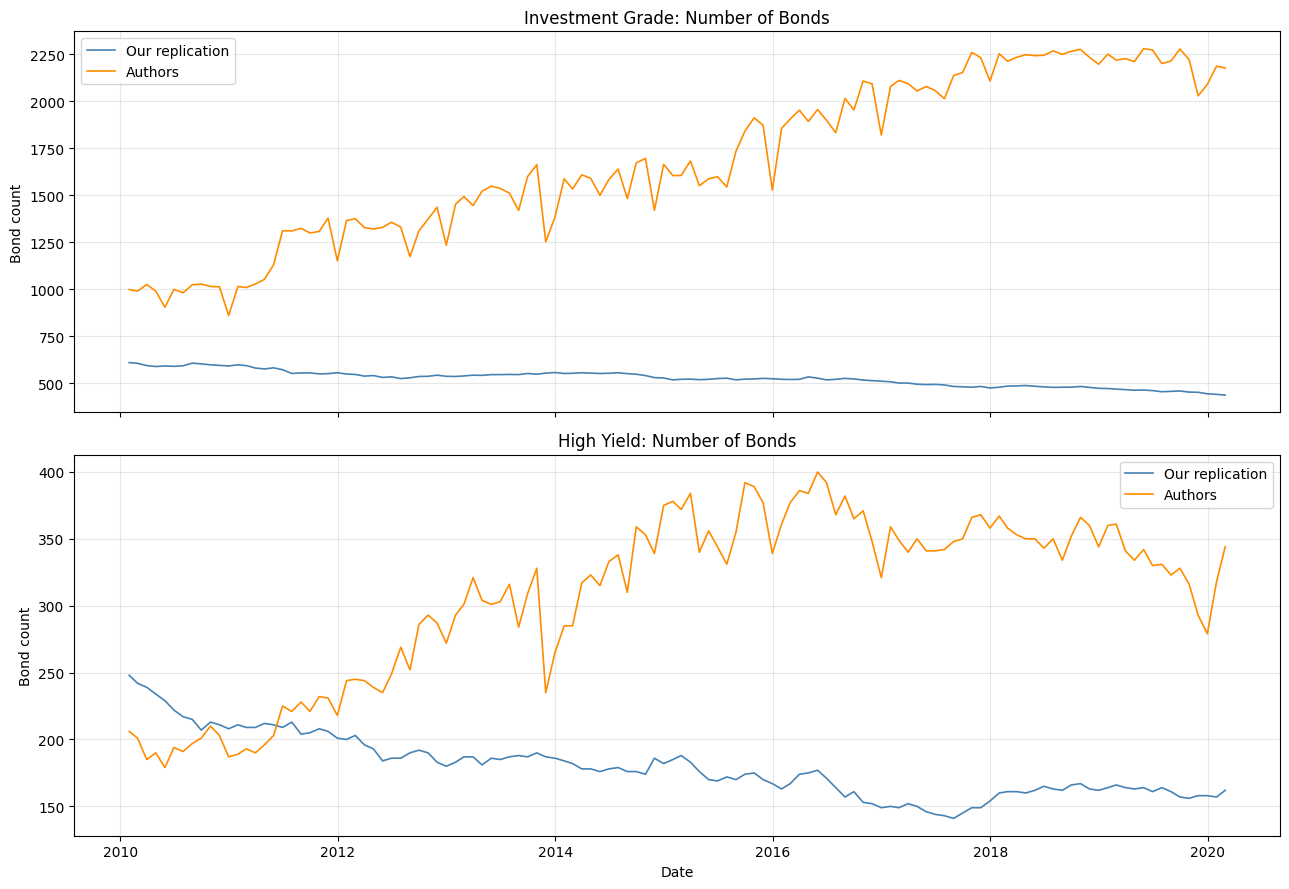
10. Comparison with Authors (Replication Window)#

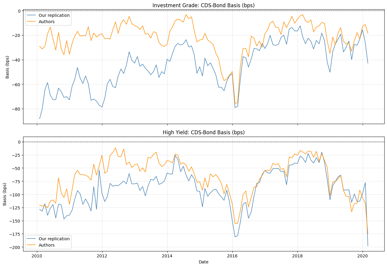
This section compares our replication to the authors’ dataset over the replication window (2010-01-01 to 2020-02-29).

Basis spread comparison in bps (monthly)
Bond-count comparison (monthly)
Side-by-side summary table (mean/median/std + bond-count moments)

authors_path = BASE_DIR / "data_manual" / "cds_paper_data.xlsx"
sheet_candidates = ["basis", "Bases"]

xl = pd.ExcelFile(authors_path)
sheet_name = next((s for s in sheet_candidates if s in xl.sheet_names), None)
if sheet_name is None:
    raise ValueError(
        f"Could not find any of {sheet_candidates} in {authors_path}. "
        f"Found sheets: {xl.sheet_names}"
    )

authors_df = pd.read_excel(authors_path, sheet_name=sheet_name).copy()
authors_df.columns = [c.strip() for c in authors_df.columns]
colmap = {c.lower(): c for c in authors_df.columns}

date_col = colmap.get("date")
basis_col = colmap.get("cds_bond_basis")
rating_col = colmap.get("ratingbin")
bond_count_col = colmap.get("bond_count")
if not all([date_col, basis_col, rating_col, bond_count_col]):
    raise ValueError(f"Unexpected authors columns: {authors_df.columns.tolist()}")

# Parse messy date values robustly.
raw_date = authors_df[date_col]
parsed_date = pd.to_datetime(raw_date, errors="coerce")
needs_serial = raw_date.notna() & parsed_date.isna()
if needs_serial.any():
    serial = pd.to_numeric(raw_date[needs_serial], errors="coerce")
    parsed_date.loc[needs_serial] = pd.to_datetime(
        serial, unit="D", origin="1899-12-30", errors="coerce"
    )

authors_df["date"] = parsed_date
authors_df["cds_bond_basis"] = pd.to_numeric(authors_df[basis_col], errors="coerce")
authors_df["bond_count"] = pd.to_numeric(authors_df[bond_count_col], errors="coerce")
authors_df["c_rating"] = (
    authors_df[rating_col].astype(str).str.strip().str.upper().map(
        {"IG": "Investment Grade", "HY": "High Yield"}
    )
)
authors_df = authors_df.dropna(subset=["date", "cds_bond_basis", "bond_count", "c_rating"]).copy()

rep_start = pd.Timestamp("2010-01-01")
rep_end = pd.Timestamp("2020-02-29")

authors_df = authors_df[(authors_df["date"] >= rep_start) & (authors_df["date"] <= rep_end)].copy()
authors_monthly = (
    authors_df.sort_values("date")
    .assign(month=lambda d: d["date"].dt.to_period("M"))
    .groupby(["month", "c_rating"], as_index=False)
    .tail(1)
    .copy()
)
authors_monthly["date"] = authors_monthly["month"].dt.to_timestamp("M")
authors_monthly["cds_basis_spread_bps"] = authors_monthly["cds_bond_basis"] * 10000.0
authors_monthly["n_bonds"] = pd.to_numeric(authors_monthly["bond_count"], errors="coerce")
authors_monthly = authors_monthly[["date", "c_rating", "cds_basis_spread_bps", "n_bonds"]]
authors_monthly = authors_monthly.sort_values(["date", "c_rating"]).reset_index(drop=True)

our_rep = agg_df.copy()
if "analysis_period" in our_rep.columns:
    our_rep = our_rep[our_rep["analysis_period"] == "replication_2010_2020"].copy()
else:
    our_rep = our_rep[(our_rep["date"] >= rep_start) & (our_rep["date"] <= rep_end)].copy()
our_rep["date"] = pd.to_datetime(our_rep["date"], errors="coerce")
our_rep = our_rep.dropna(subset=["date"]).copy()
our_rep = our_rep.sort_values(["date", "c_rating"])

print(f"Authors sheet used: {sheet_name}")
print(
    "Our replication monthly rows:", len(our_rep),
    "| Authors month-end rows:", len(authors_monthly)
)

Authors sheet used: Bases
Our replication monthly rows: 244 | Authors month-end rows: 244

def _stats_table_for_dataset(df, dataset_name):
    rows = []
    for rating in ["Investment Grade", "High Yield"]:
        sub = df[df["c_rating"] == rating].copy()
        rows.append(
            {
                "dataset": dataset_name,
                "rating": rating,
                "n_months": int(len(sub)),
                "start_date": sub["date"].min() if len(sub) else pd.NaT,
                "end_date": sub["date"].max() if len(sub) else pd.NaT,
                "mean_bps": float(sub["cds_basis_spread_bps"].mean()) if len(sub) else pd.NA,
                "median_bps": float(sub["cds_basis_spread_bps"].median()) if len(sub) else pd.NA,
                "std_bps": float(sub["cds_basis_spread_bps"].std()) if len(sub) else pd.NA,
                "mean_n_bonds": float(sub["n_bonds"].mean()) if len(sub) else pd.NA,
                "median_n_bonds": float(sub["n_bonds"].median()) if len(sub) else pd.NA,
            }
        )
    return pd.DataFrame(rows)


comparison_stats = pd.concat(
    [
        _stats_table_for_dataset(our_rep, "Our replication"),
        _stats_table_for_dataset(authors_monthly, "Authors"),
    ],
    ignore_index=True,
)
print("Replication-window comparison stats (monthly):")
display(comparison_stats)

Replication-window comparison stats (monthly):

	dataset	rating	n_months	start_date	end_date	mean_bps	median_bps	std_bps	mean_n_bonds	median_n_bonds
0	Our replication	Investment Grade	122	2010-01-31	2020-02-29	-43.852373	-42.835425	18.198621	526.713115	528.0
1	Our replication	High Yield	122	2010-01-31	2020-02-29	-88.019349	-84.569900	35.462100	179.426230	176.0
2	Authors	Investment Grade	122	2010-01-31	2020-02-29	-21.451358	-19.073266	13.029760	1683.934426	1607.5
3	Authors	High Yield	122	2010-01-31	2020-02-29	-65.978740	-61.050809	35.658357	306.139344	329.0

10.1 Basis Spread (Monthly, bps): Our Replication vs Authors#

fig, axes = plt.subplots(2, 1, figsize=(13, 9), sharex=True)
for ax, rating in zip(axes, ["Investment Grade", "High Yield"]):
    s_our = our_rep[our_rep["c_rating"] == rating].sort_values("date")
    s_auth = authors_monthly[authors_monthly["c_rating"] == rating].sort_values("date")

    ax.plot(
        s_our["date"],
        s_our["cds_basis_spread_bps"],
        label="Our replication",
        linewidth=1.2,
        color="steelblue",
    )
    ax.plot(
        s_auth["date"],
        s_auth["cds_basis_spread_bps"],
        label="Authors",
        linewidth=1.2,
        color="darkorange",
    )
    ax.axhline(0, color="black", linewidth=0.8, linestyle="--")
    ax.set_title(f"{rating}: CDS-Bond Basis (bps)")
    ax.set_ylabel("Basis (bps)")
    ax.grid(alpha=0.3)
    ax.legend(loc="best")

axes[-1].set_xlabel("Date")
plt.tight_layout()
plt.show()

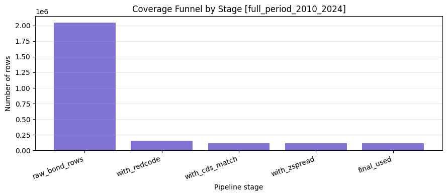
../../_images/2dfdf88f4477da26064c4485bebe1d36ed7e10815128d6ac7b8a9b348008afc1.png

Appendix A. Coverage Funnel Through the Pipeline#

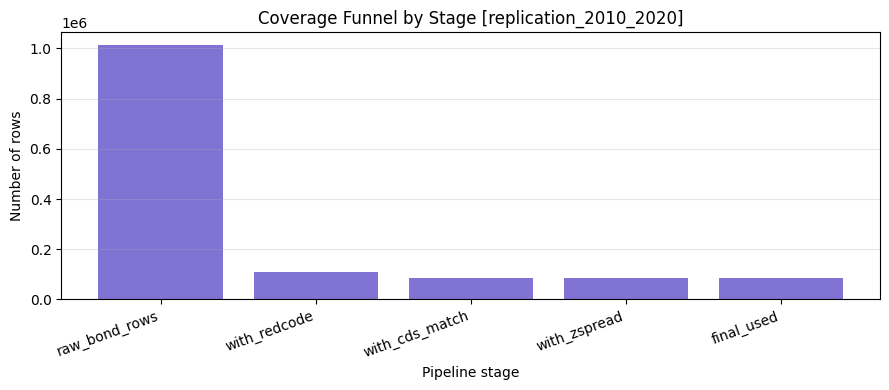
This appendix reports how many observations survive each major step:

Raw bond panel
After RED mapping
After CDS merge/interpolation
With non-missing z-spread
Final processed sample used for basis outputs

raw_bond_df = pd.read_parquet(DATA_DIR / "wrds_bondret_project.parquet")
red_df = pd.read_parquet(DATA_DIR / "red_data.parquet")
final_df = pd.read_parquet(DATA_DIR / "final_data.parquet")
z_df = pd.read_parquet(DATA_DIR / "final_data_with_z_spread.parquet")
processed_df = pd.read_parquet(DATA_DIR / "cds_basis_processed.parquet")


def _id_col(df):
    for c in ["isin", "cusip", "i_id"]:
        if c in df.columns:
            return c
    return None


def _filter_period(df, start_date, end_date):
    out = df.copy()
    if "date" not in out.columns:
        return out
    out["date"] = pd.to_datetime(out["date"], errors="coerce")
    return out[(out["date"] >= start_date) & (out["date"] <= end_date)].copy()


def _count_stage(df, stage_name):
    idc = _id_col(df)
    return {
        "stage": stage_name,
        "n_rows": int(len(df)),
        "n_unique_ids": int(df[idc].nunique()) if idc is not None else pd.NA,
    }


if {"analysis_period", "period_label", "period_start", "period_end"}.issubset(stats_df.columns):
    period_meta = (
        stats_df[["analysis_period", "period_label", "period_start", "period_end"]]
        .drop_duplicates()
        .sort_values("period_start")
        .copy()
    )
else:
    period_meta = pd.DataFrame(
        [
            {
                "analysis_period": "replication_2010_2020",
                "period_label": "Replication (2010-01-01 to 2020-02-29)",
                "period_start": "2010-01-01",
                "period_end": "2020-02-29",
            },
            {
                "analysis_period": "full_period_2010_2024",
                "period_label": "Full Period (2010-01-01 to 2024-12-31)",
                "period_start": "2010-01-01",
                "period_end": "2024-12-31",
            },
        ]
    )


for _, meta in period_meta.iterrows():
    p_name = meta["analysis_period"]
    p_label = meta["period_label"]
    p_start = pd.Timestamp(meta["period_start"])
    p_end = pd.Timestamp(meta["period_end"])

    raw_p = _filter_period(raw_bond_df, p_start, p_end)
    red_p = _filter_period(red_df, p_start, p_end)
    final_p = _filter_period(final_df, p_start, p_end)
    z_p = _filter_period(z_df, p_start, p_end)
    if "z_spread" in z_p.columns:
        z_p = z_p[z_p["z_spread"].notna()].copy()
    processed_p = _filter_period(processed_df, p_start, p_end)

    funnel = pd.DataFrame(
        [
            _count_stage(raw_p, "raw_bond_rows"),
            _count_stage(red_p, "with_redcode"),
            _count_stage(final_p, "with_cds_match"),
            _count_stage(z_p, "with_zspread"),
            _count_stage(processed_p, "final_used"),
        ]
    )
    funnel["pct_of_prev_rows"] = (funnel["n_rows"] / funnel["n_rows"].shift(1) * 100).round(2)
    funnel.loc[0, "pct_of_prev_rows"] = 100.0
    funnel["pct_of_raw_rows"] = (funnel["n_rows"] / funnel["n_rows"].iloc[0] * 100).round(2)

    print(f"Coverage funnel [{p_name}] - {p_label}")
    display(funnel)

    fig, ax = plt.subplots(figsize=(9, 4))
    ax.bar(funnel["stage"], funnel["n_rows"], color="slateblue", alpha=0.85)
    ax.set_title(f"Coverage Funnel by Stage [{p_name}]")
    ax.set_ylabel("Number of rows")
    ax.set_xlabel("Pipeline stage")
    ax.grid(axis="y", alpha=0.3)
    plt.xticks(rotation=20, ha="right")
    plt.tight_layout()
    plt.show()

Coverage funnel [replication_2010_2020] - Replication (2010-01-01 to 2020-02-29)

	stage	n_rows	n_unique_ids	pct_of_prev_rows	pct_of_raw_rows
0	raw_bond_rows	1013297	49042	100.00	100.00
1	with_redcode	110594	2298	10.91	10.91
2	with_cds_match	86270	1925	78.01	8.51
3	with_zspread	86149	1924	99.86	8.50
4	final_used	86149	1924	100.00	8.50

../../_images/1a55df53f21138035f3b366bea2dd0c15e053f9b1119d5f14b3747b721fbbde6.png

Coverage funnel [full_period_2010_2024] - Full Period (2010-01-01 to 2024-12-31)

	stage	n_rows	n_unique_ids	pct_of_prev_rows	pct_of_raw_rows
0	raw_bond_rows	2045502	115097	100.00	100.00
1	with_redcode	153943	2690	7.53	7.53
2	with_cds_match	118908	2244	77.24	5.81
3	with_zspread	118750	2243	99.87	5.81
4	final_used	118750	2243	100.00	5.81

../../_images/adb21cd3edbb24f83e3665e7957ad4e70030fb4c8d83d9cf08c6fda2b6f8c27e.png

10.2 Bond Counts (Monthly): Our Replication vs Authors#

fig, axes = plt.subplots(2, 1, figsize=(13, 9), sharex=True)
for ax, rating in zip(axes, ["Investment Grade", "High Yield"]):
    s_our = our_rep[our_rep["c_rating"] == rating].sort_values("date")
    s_auth = authors_monthly[authors_monthly["c_rating"] == rating].sort_values("date")

    ax.plot(
        s_our["date"],
        s_our["n_bonds"],
        label="Our replication",
        linewidth=1.2,
        color="steelblue",
    )
    ax.plot(
        s_auth["date"],
        s_auth["n_bonds"],
        label="Authors",
        linewidth=1.2,
        color="darkorange",
    )
    ax.set_title(f"{rating}: Number of Bonds")
    ax.set_ylabel("Bond count")
    ax.grid(alpha=0.3)
    ax.legend(loc="best")

axes[-1].set_xlabel("Date")
plt.tight_layout()
plt.show()

../../_images/f3ad3a78461c7790dad5824666ac1afc4f62516204561c4e39aef801de191fdd.png

Categories

Tags